How To Draw Indifference Curves Given Utility

The topics in this Lesson present a fleck more advanced material than was built into the previous two Microeconomics Lessons. We brainstorm with indifference curve analysis. An indifference bend is presented in Effigy 1 below.

Suppose we measure an individual's consumption of article X and commodity Y along the horizontal and vertical axes respectively and so arbitrarily selection a point in the resulting (X , Y) space such as, for case, point A. Now imagine that we label with a plus sign every point in the space that is preferred to point A and and then label with a minus sign every bespeak in the space that indicate A is preferred to. If we then draw a line that separates the plus from the minus signs, we volition obtain the indifference bend shown in the above effigy. The private will be indifferent between all combinations of Ten and Y indicated past the curve and will prefer all combinations higher up the indifference curve to any combination on the curve. And any combination along the indifference bend volition exist preferred to all combinations below it.

Since every (X , Y) combination will have an indifference curve passing through it, we tin can add together a third axis stretching upward from the bottom left corner of the figure measuring the degree to which the individual'due south preferences are satisfied, and visualize the infinitely many indifference curves as representing a smooth surface that rises as the consumption of bolt X and Y increment. Nosotros announce the caste to which preferences are satisfied as the level of utility and assume that individuals cull the combination of appurtenances X and Y, amongst those available, that maximizes their utility, with an increase in utility occurring whenever there is an increase in the quantity of either X or Y consumed, holding consumption of the other skilful constant.

Utility theory thus assumes that individuals have an internally consistent gear up of preferences that do not change during the time-interval during which we are analyzing their behaviour. In this sense we assume that individuals are rational. Irrational behaviour is illustrated in Figure 2 below.

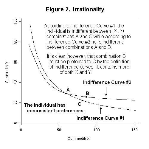
Suppose that an private has indifference curves that cross, as in the instance of Bend #1 and Curve #2 higher up. This implies that the individual is indifferent between combinations A and B and between combinations A and C. As a event, he must exist also indifferent between points B and C. But signal B has to be preferred to point C because it is above the indifference curve on which point C is located. The individual is consuming more of both appurtenances at betoken B than at bespeak C. The crossing of ii indifference curves presents a logical contradiction in the sense that the individual is behaving inconsistently or, every bit we would say, irrationally.

Economists have frequently been criticized for their assumption that people are rational. After all, we can recollect of many examples of people doing stupid things. Irrational behaviour of friends and relatives and other people nosotros observe is role of the human condition. In this respect, withal, it is of import to sympathize that economists' definition of rationality means simply that individuals deport consistently, even so stupid and irrational that consistent behaviour might announced to others. And while information technology is clear that some peoples' behaviour may exist unstable through time, the economist has to assume that the bulk of people whose behaviour is existence analyzed have unchanged preferences during the menstruation over which the analysis is taking place.

In fact, without an assumption that people have consistent preferences that do not change during the period being analyzed, no coherent analysis of social behaviour would be possible---all that would be possible is a factual delineation of what has happened in the past by historians who must carefully avoid whatever interpretation of those observed facts. Of course, psychologists and sociologists, and occasionally economists, volition attempt to determine how and why preferences change through time, but they likewise have to assume coherent and internally consistent preferences that are capable of systematic interpretation.

In the simple case portrayed in the two Figures above, economists assume that an private's utility can be expressed as a function of---that is, dependent on---the quantities of commodities X and Y consumed. Mathematically, we can write

1. U = U(X , Y)

where U is the level of utility and the office U(Ten , Y) states simply that the level of utility depends in some way on the levels of bolt X and Y consumed by the private. If we want to get fancy and analyse a state of affairs where the individual'due south preferences change, nosotros could expand the utility function by inserting between the brackets an additional input, phone call information technology Z, that measures the forces causing preferences to modify, yielding the function U(10 , Y , Z). Analytical extensions of this sort are, of class, extremely hard if not impossible to successfully pursue.

The presentation of the utility part in Equation one is extremely general---without additional specifications, the human relationship denoted by U(X , Y) could take any class. Several important features of the utility role are ever specified. First, as we noted above, increases in the levels of Ten and Y always lead to increases in U . That is, the partial derivatives of the utility role with respect to X and Y ---the changes in U associated with in pocket-size changes in each of X and Y belongings the other abiding---are positive. Mathematically, this imposes the two atmospheric condition

2. ∂U/∂X = ∂U(X , Y)/∂10 > 0 and ∂U/∂Y = ∂U(Ten , Y)/∂Y > 0

where ∂U/∂X is the fractional derivative of U(X , Y) with respect to X and ∂U/∂Y is the partial derivative with respect to Y. Nosotros refer to ∂U/∂X and ∂U/∂Y as, respectively, the marginal utility of X and the marginal utility of Y. Equations 2 specify that marginal utilities of X and Y are positive.

The second specified feature of the office U(X , Y) is the principle of diminishing marginal utility. This says that the marginal utility of X declines equally the quantity of X increases and the marginal utility of Y declines equally the quantity of Y increases. The gradient of an indifference bend is the negative of the ratio of the marginal utility of X over the marginal utility of Y. To see this, imagine that the quantities of X and Y change by modest amounts. The change in utility specified in Equation 1 tin can then be expressed mathematically equally

3. dU = ∂U(X , Y)/∂Ten dX + ∂U(X , Y)/∂Y dY = ∂U/∂X dX + ∂U/∂Y dY

where the letter d preceding a variable denotes a small change in that variable. Since the level of utility must be constant---that is dU = 0 ---along an indifference bend, Equation 3 can be rearranged to yield

0 = ∂U/∂X dX + ∂U/∂Y dY

which can be further rearranged as

4. dY/dX = − ∂U/∂X / ∂U/∂Y

where dY/dX is the slope of the indifference curve. The principle of diminishing marginal utility implies that ∂U/∂X , the marginal utility of X, falls as the quantity of X consumed increases and that ∂U/∂Y , the marginal utility of Y, rises as the quantity of Y consumed decreases. Every bit tin can be seen from Equation 4, this implies that the indifference bend gets flatter as the quantity of X consumed increases relative to the quantity of Y consumed. Or, every bit we say, indifference curves are concave outward, or convex with respect to the origin. The slope of the indifference curve is called the marginal charge per unit of commutation, which declines equally the quantity of X increases relative to the quantity of Y.

Of course, the amounts of commodities X and Y that the individual volition be able to consume depends on the level of that person's income. If the entire income is spent on article X, the maximum quantity that tin can be consumed is given past the distance between the origin and indicate B on the horizontal axis of Figure 3 below. If the entire income is spent on commodity Y, the maximum quantity that can exist consumed is given by the vertical distance between the origin and indicate A. If the prices of the ii bolt facing the individual are constant, the ratio of the toll of article X to the price of commodity Y is given by the slope of the budget line running from point A to bespeak B.

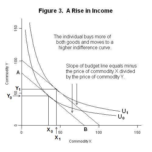
The optimal quantities consumed will be that combination of X and Y that puts the private on the highest possible indifference bend---that is, quantities 10₀ and Y₀ on the to a higher place Figure. Note that the equilibrium quantities are those for which the slope of the indifference curve equals the slope of the budget line---that is, where the marginal rate of substitution equals the price ratio.

Now suppose that the level of the individual'south income increases without whatsoever alter in prices. More of both commodities tin at present be consumed and the price ratio does not change, so the budget line shifts outward with the new budget line beingness parallel to the original 1. The level of utility increases from U₀ to U_i and the individual's consumption of the two appurtenances increases to X₁ and Y_one . At this point nosotros must continue in mind that the indifference map in Figure 3 assumes that both X and Y are normal goods---that is, that indifference curve U₁ is tangent to the new college budget line at a indicate to the right of output level X₀. In the case where X is an inferior good, this tangency would be to the left of output level X₀ and the quantity demanded of commodity X would refuse every bit a result of the increase in income.

Finally, let the states suppose that the cost of commodity X falls, with no modify in money income. The results are shown in Effigy 4 beneath.

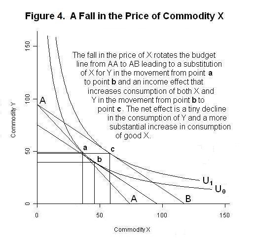
If the individual were to spend his entire income on commodity Ten, the amount of 10 purchased would now exist higher. Since the price of practiced Y has not inverse, neither has the maximum possible consumption of that commodity. The fall in the price of X has thus reduced the slope of the individual's upkeep line past rotating it counter-clockwise around point A on the vertical axis. The new utility maximum occurs at point c with a big increase in the quantity of good 10 consumed and a slight pass up in consumption of good Y.

Information technology is important to distinguish between two components of the shift from the initial equilibrium point to the final equilibrium at betoken c---the income effect and the substitution result. The decline in the toll of X leads to a substitution of good X for good Y along the initial indifference curve, holding real income---that is utility---constant. This substitution effect is indicated by the movement from combination a to combination b along indifference bend U₀. The fact that real income has increased as a consequence of the reject in the price of good X, belongings nominal income and the price of good Y constant, results in an increase in the quantities consumed of both goods, represented past the move from combination b to combination c. This income effect is represented by the motility from indifference curve U₀ to U_ane. As you lot tin can see from the to a higher place Effigy, the quantity consumed of good 10 increases as a event of both the exchange and income effects while the quantity of skillful Y consumed declines as a effect of the substitution result and increases by slightly less than that amount as a result of the income event, leaving a slight overall decline.

It should now be clear why demand curves gradient down when the goods, every bit in the higher up analysis, are substitutes for each other. It is obvious from Figure 4 that a fall in the toll of commodity X, holding nominal income constant, results in an increase in the need for that good. In that Figure, the fall in the price of good X as well shifts the demand curve for good Y slightly to the left because the substitution effect more than offsets the result of the pass up in real income. Besides, it is clear from Figure 3 that an increase in nominal income, holding prices constant, shifts the need curves of both appurtenances to the right and, therefore, that both commodities in that example are superior goods.

In the real world, each individual volition spend her income on many appurtenances in each flow of her life, and volition face relative prices that may modify from period to menstruum along with the involvement rate, which measures the cost of consuming in the present equally opposed to future periods. In a world where consumption externalities are present, she may also experience gains and losses in utility from the behaviour of others over which she has no control. This means that more advanced assay will involve a utility office with many more arguments. On the ground of our two-commodity analysis above, however, it is reasonable to look that the marginal rate of substitution of each good for each other in the utility office will, in equilibrium, equal the relative price of that pair of appurtenances. The principles of diminishing marginal utility and diminishing marginal rate of commutation can reasonably be causeless to be widely applicable.

It is at present time for a exam. As ever, think up your ain answers before looking at the ones provided.

Question i
Question 2
Question 3